NIRSimple example

→ Download this notebook

import scipy.io
import numpy as np
import nirsimple as ns

The data used in this example is from the Homer MATLAB toolbox tutorial and can be downloaded here.

Download the zip archive and extract it. In this example we are just going to use Simple_Probe.nirs which is in the Example1_Simple_Probe folder of the archive.

Load data from the file

Load the file as a MATLAB file:

file_path = "./Simple_Probe.nirs"  # replace by the path to Simple_Probe.nirs
simple_probe = scipy.io.loadmat(file_path)

Get fNIRS light intensities as a numpy array

Get signals from Simple Probe:

intensities = np.swapaxes(simple_probe['d'], 0, 1)
print("Intensity data shape: {}".format(intensities.shape))
print("  number of channels: {}".format(intensities.shape[0]))
print("  number of time points: {}".format(intensities.shape[1]))

Intensity data shape: (8, 1200)
  number of channels: 8
  number of time points: 1200

Convert light intensities to optical density changes

Get optical density changes relative to the average intensity of each channel:

dod = ns.intensities_to_od_changes(intensities)
print("Delta OD shape: {}".format(dod.shape))

Delta OD shape: (8, 1200)

Get channel info as lists

Get channel names from Simple Probe:

channels = simple_probe['SD']['MeasList'][0, 0][:, :2].tolist()
raw_ch_names = [str(ch).replace('[', '').replace(']', '').replace(', ', '-')
                for ch in channels]
print("Channel names: {}".format(raw_ch_names))

Channel names: ['1-1', '1-2', '1-3', '1-4', '1-1', '1-2', '1-3', '1-4']

---

Get channel wavelengths from Simple Probe:

wavelengths = simple_probe['SD']['Lambda'][0, 0][0].tolist()
ch_high_wl = [wavelengths[0] for _ in range(int(len(raw_ch_names)/2))]
ch_low_wl = [wavelengths[1] for _ in range(int(len(raw_ch_names)/2))]
ch_wl = ch_high_wl + ch_low_wl
print("Channel wavelengths: {}".format(ch_wl))

Channel wavelengths: [830, 830, 830, 830, 690, 690, 690, 690]

---

Define the differential pathlengths factor (DPF) for each channel:

unique_dpf = 6
ch_dpf = [unique_dpf for _ in enumerate(raw_ch_names)]
print("Channel DPFs: {}".format(ch_dpf))

Channel DPFs: [6, 6, 6, 6, 6, 6, 6, 6]

---

Define source-detector distance for each channel:

unique_distance = 2.8  # cm
ch_distances = [unique_distance for _ in enumerate(raw_ch_names)]
print("Channel distances: {}".format(ch_distances))

Channel distances: [2.8, 2.8, 2.8, 2.8, 2.8, 2.8, 2.8, 2.8]

Convert optical density changes to concentration changes

Get oxygenated and deoxygenated hemoglobin concentration changes (HbO and HbR) with the modified Beer-Lambert law (from Delpy et al., 1988):

data = ns.mbll(dod, raw_ch_names, ch_wl, ch_dpf, ch_distances,
               unit='cm', table='wray')
dc, ch_names, ch_types = data
print("Delta HbO and HbR shape: {}".format(dc.shape))
print("Channel names: {}".format(ch_names))
print("Channel types: {}".format(ch_types))

Delta HbO and HbR shape: (8, 1200)
Channel names: ['1-1', '1-1', '1-2', '1-2', '1-3', '1-3', '1-4', '1-4']
Channel types: ['hbo', 'hbr', 'hbo', 'hbr', 'hbo', 'hbr', 'hbo', 'hbr']

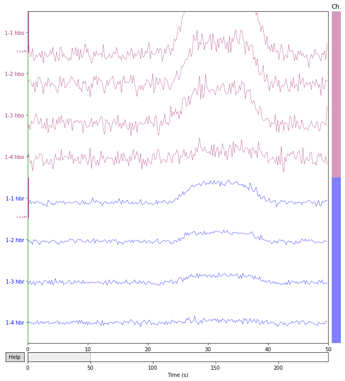
Plot data with MNE

import mne

S_FREQ = 5  # sampling frequency in Hz

Plot data with MNE:

mne_ch_names = [ch + ' ' + ch_types[i] for i, ch in enumerate(ch_names)]
print("MNE channel names: {}".format(mne_ch_names))
info = mne.create_info(ch_names=mne_ch_names, sfreq=S_FREQ,
                       ch_types=ch_types)
raw = mne.io.RawArray(dc, info)
graph = raw.plot(scalings=0.5e-6, duration=50)

MNE channel names: ['1-1 hbo', '1-1 hbr', '1-2 hbo', '1-2 hbr', '1-3 hbo', '1-3 hbr', '1-4 hbo', '1-4 hbr']
Creating RawArray with float64 data, n_channels=8, n_times=1200
    Range : 0 ... 1199 =      0.000 ...   239.800 secs
Ready.

Signal correction

Apply correlation based signal improvement (from Cui at al., 2010) to hemoglobin concentration changes:

data = ns.cbsi(dc, ch_names, ch_types)
dc_0, ch_names_0, ch_types_0 = data
print("Delta HbO_0 and HbR_0 shape: {}".format(dc_0.shape))
print(ch_names_0)

Delta HbO_0 and HbR_0 shape: (8, 1200)
['1-1', '1-1', '1-2', '1-2', '1-3', '1-3', '1-4', '1-4']

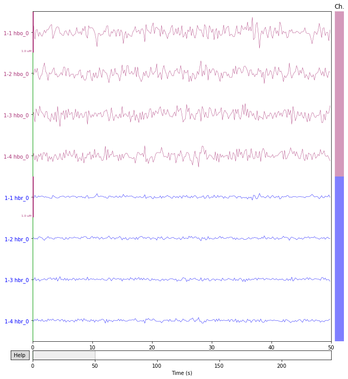
Plot corrected data with MNE

mne_ch_names_0 = [ch + ' ' + ch_types_0[i] + '_0'
                  for i, ch in enumerate(ch_names_0)]
print("MNE channel names: {}".format(mne_ch_names_0))
info_0 = mne.create_info(ch_names=mne_ch_names_0, sfreq=S_FREQ,
                         ch_types=ch_types_0)
raw_0 = mne.io.RawArray(dc_0, info_0)
graph_0 = raw_0.plot(scalings=0.5e-6, duration=50)

MNE channel names: ['1-1 hbo_0', '1-1 hbr_0', '1-2 hbo_0', '1-2 hbr_0', '1-3 hbo_0', '1-3 hbr_0', '1-4 hbo_0', '1-4 hbr_0']
Creating RawArray with float64 data, n_channels=8, n_times=1200
    Range : 0 ... 1199 =      0.000 ...   239.800 secs
Ready.